I took the fast.ai course to get a practical handle on machine learning. The course cuts through academic gatekeeping and focuses on building working models first, then understanding theory. These are my notes from that journey, covering random forests, neural networks, and deep learning with convolutional neural networks.
The Two Pillars of Modern ML
Modern machine learning can be distilled down to two techniques that cover the majority of use cases:
Ensembles of decision trees like random forests and gradient boosting machines work best for structured data — anything that fits neatly into rows and columns.
Multi-layered neural networks trained with stochastic gradient descent handle unstructured data like audio, images, and natural language.
ML problems themselves fall into two camps. Regressors predict continuous variables like price. Classifiers predict categories like whether an image contains a cat or a dog. The variable you’re trying to predict is called the dependent variable.
Evaluation Functions
Before building a model, you need a way to measure how well it predicts. Several evaluation functions exist for this purpose.
Root Mean Square Error
$$ RMSE = \sqrt{ {\frac{1}{N}\sum_{i=1}^N(actual_i - prediction_i)^2}} $$
RMSE gives you a single number representing prediction error in the same units as your target variable. Larger errors are penalized more heavily because of the squaring.
Root Mean Square Log Error
$$ RMSLE = \sqrt{ {\frac{1}{N}\sum_{i=1}^N(\log(actual_i) - \log(prediction_i))^2}} $$
Taking logs means errors in predicting expensive items and cheap items affect the score equally. Without logs, a large error on a high-value item would dominate a small error on a low-value item.
Coefficient of Determination
$R^2$ ranges from $-\infty$ to 1, where 1 indicates a perfect prediction. A negative value means the model is worse than simply predicting the mean. It’s a ratio of how good the model is compared to a naive mean model.
Preparing Data for Random Forests
Random forests need numbers. They can’t work with strings or dates directly. The fast.ai library provides several utilities to handle this.
add_datepart breaks date columns into useful components: year, month, day, day of week, and more. This lets the model learn seasonal patterns and trends. train_cats converts string columns into pandas categories, which can then be accessed as integer codes via cat.codes. Finally, proc_df turns everything into numbers — missing continuous values get replaced by the median, and a boolean _na column is added to flag which rows had missing data.
How Decision Trees Choose Split Points
A decision tree works by recursively splitting the data. At each node, the algorithm runs through every possible variable and every possible split point. It picks the split where the weighted average of mean squared error times sample count is lowest. An equivalent approach is finding the split where both groups have the lowest weighted standard deviation.
The process repeats recursively for the subsets on each side of the split until no more useful splits are possible. A random forest builds many of these trees, each trained on a different subset of the data, and averages their predictions.
Picking a Validation Set
Random selection works for most datasets, but breaks down when there’s a temporal factor. If you’re predicting future values, the validation set should contain the most recent data while the model trains on everything before it. This simulates how the model will actually be used.
A useful sanity check: build five models, score each on both validation and test sets, then plot the results. The points should fall roughly on a line. If they don’t, the validation set isn’t representative of the test set.
Out-of-Bag Score
Each tree in a random forest uses a different subset of the training data — a process called bagging. The OOB score takes advantage of this. For each training row, it calculates the error using only the trees where that row wasn’t part of the training subset. This gives a validation-like score without needing a separate validation set.
OOB scores are always slightly worse than validation set scores because they only use a subset of the forest for each prediction. Still, they’re useful when data is scarce.
Random Forest Hyperparameters
Three key hyperparameters control the trade-off between accuracy and generalization.
Subsampling (set_rf_samples) controls how many rows each tree trains on. Fewer rows means less overfitting but also less accuracy per tree. The goal is to make each estimator accurate while keeping correlation between estimators low.
Min samples leaf sets the minimum number of records in each leaf node. Increasing it effectively removes one level from each tree ($\log_2(20000) - 1$). Individual trees become less accurate but also less correlated with each other.
Max features limits how many randomly selected features each split can consider. Fewer features means more varied trees. Without this constraint, every tree would split on the same highly predictive feature first, making the forest less diverse.
Feature Importance
Understanding which features matter most is often more valuable than the predictions themselves. Random forests make this straightforward.
Run the validation set through the model and record the $R^2$. Then take a single column and randomly shuffle its values — this destroys any relationship between that feature and the dependent variable. Run the shuffled data through the model and record the new $R^2$. The drop in score is that feature’s importance. Repeat for every column.
Features that cause a large drop when shuffled are important. Features that cause little or no drop can likely be removed.
Removing Redundant Features
Highly correlated features add noise without contributing new information. Plot the rank correlation between features and identify groups of similar ones. Remove one feature from each correlated group, retrain, and watch the OOB score. If it holds steady or improves, the removed features were redundant.
Partial Dependence Plots
Feature importance tells you which features matter but not how they affect predictions. Partial dependence plots fill this gap. Replace a single feature with a constant value across all rows, run predictions through the trained model, then repeat for every value in that feature’s range.
The result shows the effect of a single feature on predictions, all else being equal. Plotting thin lines for individual records and a bold line for the mean reveals both the average effect and how it varies across the dataset.
Tree Interpreter
Sometimes you need to understand why the model made a specific prediction. The tree interpreter traces a single observation through the forest. It starts with the bias — the mean prediction for the entire training set — and after each split records the difference. The result shows exactly how the model arrived at its prediction, often visualized as a waterfall chart.
Neural Networks
Moving from random forests to neural networks is a shift from structured to unstructured data. A neural network is an infinitely flexible function made up of layers. Each layer applies a linear function (matrix multiplication) followed by a non-linear function (activation).
Linear Functions
The simplest neural network operation is the linear function:
$y = ax + b$
Here $a$ is the weight matrix and $b$ is the bias. For multiple inputs this becomes:
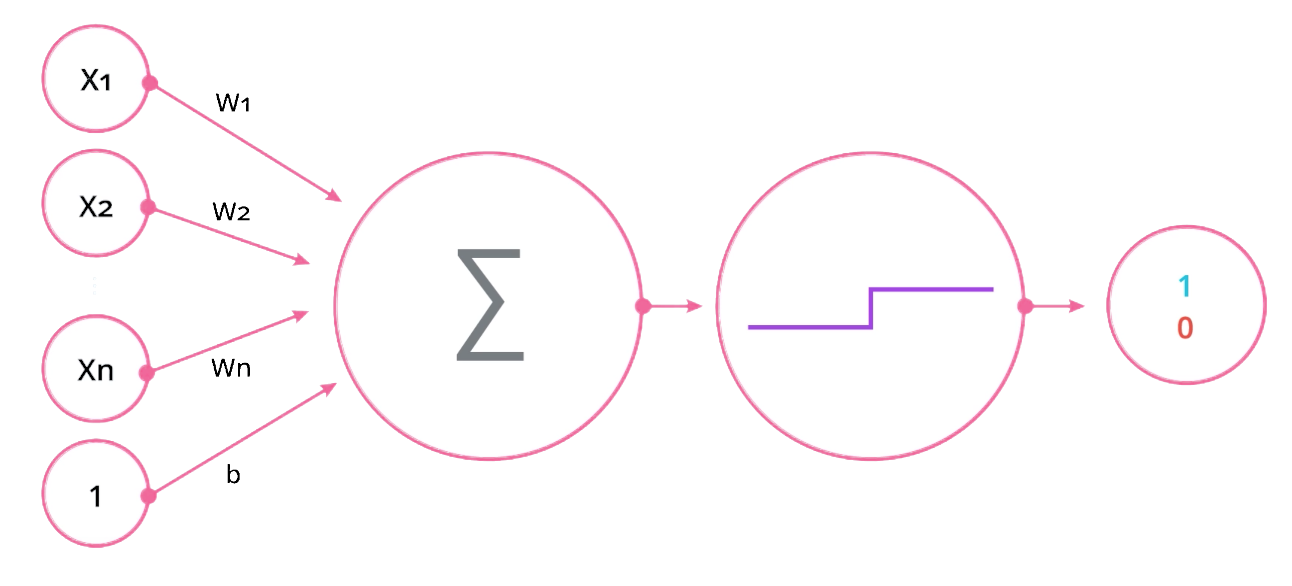
$$ \begin{aligned} &w_1x_1 + w_2x_2 + b = 0 \\ &Wx + b = \sum_{i=1}^n W_i X_i + b \end{aligned} $$
The classic perceptron illustrates this — inputs are multiplied by weights, summed with a bias, then passed through an activation function.
Activation Functions
The non-linear part of each layer is the activation function. Without non-linearity, stacking layers would be pointless — multiple linear functions collapse into a single linear function.
Softmax is typically the last layer in a classification network. It converts raw outputs into probabilities that sum to 1. Sigmoid squashes values between 0 and 1, useful for binary classification. ReLU (Rectified Linear Unit) is simply $\max(0, x)$ — it’s the most common activation for hidden layers because it’s fast and avoids vanishing gradients. Leaky ReLU is a variant that allows a small gradient when the input is negative.
The universal approximation theorem states that a neural network can approximate any function to arbitrary accuracy, given enough neurons. The practical challenge is finding the right weights.
Loss Functions
Loss functions measure how wrong the model’s predictions are. Lower is always better.
For classification problems, cross entropy (also called negative log likelihood) is the standard choice. It comes in two flavors: binary cross entropy for two-class problems and categorical cross entropy for multi-class problems.
Gradient Descent and Backpropagation
Training a neural network means finding the point of minimal loss. The derivative of the loss function indicates how much total loss changes when you adjust weights by a small amount. Backpropagation uses the chain rule to calculate these derivatives efficiently through all layers.
For a two-layer network, the feed-forward pass looks like:
$$ \hat{y} = \sigma \circ W^{(2)} \circ \sigma \circ W^{(1)}(x) $$
Each layer applies its weights, then an activation function $\sigma$, passing results to the next layer.
Cross Entropy in Depth
The probability of all data points being correctly classified is a product of individual probabilities. Multiplying many small probabilities together produces tiny numbers that computers struggle with. The solution is to use logarithms because $\log(ab) = \log(a) + \log(b)$ — multiplication becomes addition.
Since the natural log of a probability (a number between 0 and 1) is always negative, cross entropy is defined as the sum of negative log probabilities. Minimizing cross entropy is equivalent to maximizing the probability of correct predictions.
Regularization and Weight Decay
Overfitting happens when a model memorizes training data instead of learning general patterns. Regularization combats this by penalizing large coefficients — preventing any single feature from having too much explanatory power.
$$ Cost = \frac{1}{n}\sum_{i=1}^n(\hat{y}_i - y_i)^2 + \lambda\sum_{i=0}^1\beta_i^2 $$
The hyperparameter $\lambda$ controls how aggressively large coefficients are penalized. Higher $\lambda$ means simpler models. L1 regularization uses the absolute value of coefficients, while L2 uses the square. L2 is more common in practice and is often called weight decay.
Embeddings
Categorical variables are best represented as embeddings rather than raw numbers. An embedding is a learned weight matrix multiplied by a one-hot encoded input. The network learns a dense representation for each category during training.
This matters because integer encoding implies an ordering that may not exist — category 3 is not inherently “more” than category 1. Embeddings let the network learn the actual relationships between categories.
Deep Learning and Convolutional Neural Networks
Deep learning applies the same principles as basic neural networks but with more layers and specialized architectures. For image recognition, convolutional neural networks (CNNs) are the dominant approach.
Convolutions
A convolution is the result of multiplying each 3x3 grid of pixels with a 3x3 kernel (also called a filter). The kernel values are learned through gradient descent. The architecture of a CNN is defined by the number and size of its kernels.
Early kernels learn simple patterns like edges and gradients. Deeper kernels combine these into increasingly complex features — corners, textures, and eventually recognizable objects.
Stochastic Gradient Descent
SGD is the workhorse of deep learning. Rather than computing the gradient over the entire dataset, it processes small random batches (mini-batches). This is faster and introduces noise that helps escape local minima.
Learning Rates
Finding the right learning rate is one of the most important decisions in training. An epoch is one complete pass through the training data. Too high a learning rate causes the model to overshoot minima. Too low and training takes forever or gets stuck.
The fast.ai library uses cosine annealing — as the model approaches a minimum, the learning rate is gradually reduced. SGD with restarts resets the learning rate periodically, allowing the model to escape shallow minima and find better ones. The cycle_len parameter controls how many epochs per cycle, while cycle_mult multiplies the cycle length after each restart.
Data Augmentation
Transforming training images — rotating, flipping, cropping, adjusting brightness — creates additional training data for free. This is a powerful technique for combating overfitting, which manifests as training loss being much lower than validation loss.
Transfer Learning
Training a CNN from scratch requires enormous amounts of data. Transfer learning sidesteps this by starting with a pre-trained model (typically trained on ImageNet) and adapting it to your specific problem.
The process works in two stages. First, freeze the pre-trained layers and train only the final fully connected layer on your data. Then unfreeze the earlier layers and fine-tune the entire network with differential learning rates — lower rates for early layers (which capture general features) and higher rates for later layers (which need to specialize).
The weights in kernels and fully connected layers are what’s trained. Activations are values calculated from those weights during the forward pass.
Dropout
Dropout randomly discards activations during each mini-batch of training. This forces the network to learn redundant representations — no single neuron can become a crutch. A dropout probability of 0.5 means half the activations are zeroed out each pass.
High dropout improves generalization but reduces training accuracy. Low dropout provides less regularization. The right value depends on the specific problem and how much overfitting you observe.
Multi-label Classification
Standard classification picks one label per input. Multi-label classification identifies multiple things — for example, recognizing several objects in a single image.
Softmax is designed to pick one winner, so it doesn’t work for multi-label problems. Sigmoid activation handles this instead, outputting independent probabilities for each label.
Practical Troubleshooting
If the learning rate finder produces erratic results, the dataset may be too small for the current mini-batch size. Reducing the batch size often resolves this. Monitoring the gap between training and validation loss remains the most reliable way to diagnose overfitting throughout training.
Conclusion
The fast.ai course demonstrates that practical machine learning doesn’t require a PhD in statistics. Random forests handle structured data well and offer interpretability through feature importance and partial dependence plots. Neural networks extend into unstructured territory with the flexibility to approximate any function. Deep learning with CNNs and transfer learning makes image recognition accessible even with limited data.
The common thread across all three approaches is the same: define a loss function, find the parameters that minimize it, and validate against data the model hasn’t seen.